Derivation of the continuous-time Price equation

June 26, 2012

The standard discrete-time Price equation is really useful, but its derivation is much less beautiful than the continuous-time version in my opinion. The beautiful thing about the continuous-time version is that it can be used to illustrate the clear relationship between the Price equation and the chain rule.

Model and notation

Consider a set of groups of individual organisms and label the groups with $i = 1, 2, ...$ . Groups are characterized by a particular trait; every individual belonging to group $i$ is characterized by the same trait-value, $x_i$ . The number, $n_i$ , of individuals in group $i$ changes with time according to the equation,

where $r_i$ is the per capita growth rate of the $i$ th group, which may itself change over time.

Objective

Given this model, our goal is to derive an equation for the time dynamics of the weighted average of the trait, which is defined as,

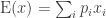
where,

is the relative abundance of the $i$ th group.

The chain rule

As I mentioned earlier, the continuous-time Price equation is essentially a special case of the chain rule. In particular, by the chain rule we can write the time-derivative of the weighted average trait value as,

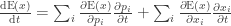
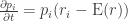
Substituting the partial derivatives of the weighted average trait value,

or with dots,

This is the most important equation in the post. Essentially its the continuous-time Price equation, but in a non-standard form. The first summation gives the selection effect: it will be large if groups with high trait values tend to be increasing in relative abundance. The second summation gives the trait dynamics effect: it will be large if abundant groups tend to be increasing in their trait values. What I like about this form of the Price equation is that it demonstrates a deep connection between evolutionary biology and many other general equations in science that are also based on the chain rule (e.g. Hamilton’s equations). The rest of the post will be about how to get from this ‘chain-rule form’ to the standard ‘moment form’.

Aside: relative abundance dynamics

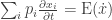
Before getting to the standard form, we need another result. The chain-rule shows up again,

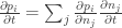
The first partial in each term comes from differentiating the definition for the relative abundances (we need the quotient rule here),

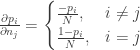
where $N = \sum_i n_i$ is the total abundance. After (as people tend to say) `some’ algebra,

which implies, given our definition of weighted averaging (i.e. mathematical expectation),

This says that groups with per capita growth rates greater than the average will increase in relative abundance, which makes sense.

Selection and covariance

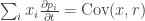
This is the title of Price’s original article. It refers to the mathematical equivalence between the concept of selection from evolutionary theory and the concept of covariance from probability theory. The original work by Price was in discrete-time. Here I’m interested in continuous-time and the chain rule. Using the time-derivative of the relative abundance derived above, we find that the first term of the Price equation can be expressed as,

Again using weighted averaging,

From the definition of covariance,

Average trait-value dynamics

Now for the second term of the continuous-time Price equation. Basically, its just the weighted average trait dynamics,

where $\dot{x_i} = \frac{\partial x_i}{\partial t}$ .

Standard form of the continuous-time Price equation

Putting all this together gives,

So…the rate of trait evolution depends on (1) the covariance between the trait and per capita growth rate and (2) the expected rate of change of the trait values. This is a beautiful equation but the chain-rule form is also beautiful, and should get more air time. Here it is again:

Hope I didn’t mess anything up! Further reading here (scroll down to the Day and Gandon 2005 book chapter). Also, Jeremy Fox of the Oikos blog has some great Price-equation-esque work in ecology (e.g.).

UPDATE: Check out the great references below that commenters have pointed out.

15 Comments leave one →

Jeremy Fox permalink

August 2, 2012 10:10 pm

This is very useful, even for a supposed Price equation “expert” like me. Because I’ve only ever had occasion to use to the discrete time Price equation in my own work, I’ve never really sat down and worked my way through the continuous time version. Steve Ellner’s recently done some nice stuff with the continuous time version in Ecology Letters, using it as a way to partition ‘evolutionary’ and ‘ecological’ changes in mean phenotype over time.

Reply
- stevencarlislewalker permalink*
  
  August 2, 2012 10:28 pm
  
  I had been hoping you’d find this! Glad you found it useful. I had been playing around with some simple models of functional diversity dynamics, and found that I was just re-discovering the continuous-time Price equation. One of these days I’ll catch up to the state of the art! Thanks for the Ellner reference too. I think I saw him presenting that stuff at ESA one year but never got around to looking at the paper.
  
  Reply
  - Jeremy Fox permalink
    
    August 2, 2012 10:48 pm
    
    If memory serves, Norberg et al. (PNAS 2000 or 2001?) is another application of the continuous time Price equation (specifically, the special case of Fisher’s Fundamental Theorem), in an ecological context. Norberg et al. were interested in how a diverse set of species can better “track” environmental fluctuations than any single species and so maintain higher total biomass on average, basically by harboring variation on which selection can act.
  - jeff smith permalink
    
    August 4, 2014 7:32 pm
    
    Another application of the continuous-time version of the Price Equation: I used it to track symbionts as characters that can be inherited vertically from one’s parents or horizontally from other individuals in a population (Am Nat 2007 170:542).
Amy Hurford permalink

August 12, 2012 12:28 pm

Another good reference is ‘Applying population-genetic models in theoretical evolutionary epidemiology’ by Troy Day and Sylvain Gandon. It’s also from Ecology Letters.

Reply
- stevencarlislewalker permalink*
  
  August 12, 2012 3:34 pm
  
  Thanks for this great reference…I’m going to give it a close reading as soon as I have some time.
  
  Reply
- Jeremy Fox permalink
  
  August 13, 2012 6:15 pm
  
  As long as we’re forcing you to read everything cool that everyone’s ever done with the Price equation…
  
  Kerr and Godfray-Smith 2009 Evolution. Extending the (discrete) Price equation to handle immigration into the descendant population.
  
  Steven Frank’s recent review in the Journal of Evolutionary Biology. Sincerely flattered to have had some of my stuff cited in that one.
  
  Reply
Michael permalink

November 11, 2014 5:43 pm

Can you not just use the product rule from the off and skip the chain rule to derive the main equation?

Reply
- stevencarlislewalker permalink*
  
  November 11, 2014 5:53 pm
  
  Yes. Well … the sum rule followed by the product rule, which are both special cases of the chain rule. But yes, I was probably being overly complex.
  
  Reply
  - Michael permalink
    
    November 12, 2014 1:49 pm
    
    Thanks Steven, just thought I would check I wasn’t missing the point. If you could help me understand a couple of other points I would really appreciate it! I am getting a bit lost at the start of the section ‘Aside: relative abundance dynamics’.
    
    1) In the chain rule for dpi/dt, where does the sum_j come from?
    
    2) I always end up with an N^2 in the denominator following the quotient rule. I have a derivative of N in the numerator, but I don’t see why it cancels.
    
    3) I’m also unsure how you then used the ‘some algebra’ following the expression for dpi/dnj.
    
    Thanks!
    
    Michael
  - stevencarlislewalker permalink*
    
    November 12, 2014 5:57 pm
    
    1) This is a ‘total derivative’:
    
    2&3) Now that I think about, its probably easier to use the product rule on:
    
    $n_i = p_i N$
    $\frac{dn_i}{dt} = \frac{dp_i}{dt} N + p_i\frac{dN}{dt}$
    $\frac{dp_i}{dt} = \frac{1}{N}\left[\frac{dn_i}{dt} - p_i\frac{dN}{dt}\right]$
    $\frac{dp_i}{dt} = \frac{1}{N}\left[r_in_i - p_i\sum_j r_jn_j\right]$
    $\frac{dp_i}{dt} = \left[r_ip_i - p_i\sum_j r_jp_j\right]$
    $\frac{dp_i}{dt} = \left[r_ip_i - p_iE(r)\right]$
    $\frac{dp_i}{dt} = p_i\left[r_i - E(r)\right]$
Michael permalink

November 13, 2014 9:25 am

Thanks Steven!

Reply
mlachmann permalink

February 23, 2017 11:02 pm

Very nice derivation. There is a tiny typo: I think that in the two equations below “chain rule”, it should be dp/dt, dx/dt full derivatives, not partial. (Though it seems wikipdeia on chain rule also has the same mistake). See, for example http://mathworld.wolfram.com/Derivative.html eq 45. If the derivative on the left hand side is partial, then you end with partials on the right, and if the derivative is full on left, you end with full on right. But this is really nitpicking.

Reply